Discrepancies Between Free-Surface Methods: ALE and Sticky Air Method in annulus models

Hello everyone,

I am using ASPECT to implement a 2D pure viscous annulus model with the free surface boundary condition applied to the top boundary. The model includes three layers: the crust, lithospheric mantle, and convecting mantle. The density of the crust is 3000 kg/m³, and the density of the lithospheric and asthenospheric mantle is 3500 kg/m³. The viscosity of the convecting mantle is 1×10²⁰ Pa·s, while that of the crust and lithospheric mantle is 1×10²⁴ Pa·s.

The model does not consider thermal effects, and crustal thickness perturbation serves as the sole driving force. Initially, the crust within a ~85 degree region is 20 km thicker than the surrounding crust, and the top surface is flat. Due to the low density of the crust, this thick crust region uplifts, drives mantle convection, and deforms the lithosphere.

I implemented the free surface boundary condition using two different methods: ALE (Arbitrary Lagrangian-Eulerian) and sticky air, but observed completely different results under identical model setups. For example, the lithospheric stress regime and mantle convection direction are totally different at ~2 million years.

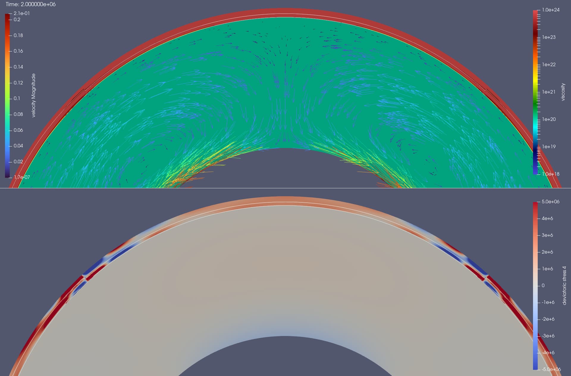
Figure 1. Viscosity (top panel) and horizontal normal deviatoric stress (bottom panel) for the ALE method at 2 myr. The velocity vectors are superimposed on the top panel. The thickened crustal region (central part of the figure) is associated with horizontal compression and downwelling flow.

Figure 2. Viscosity (top panel) and horizontal normal deviatoric stress (bottom panel) in the stick air method at 2 myr. The velocity vectors are superimposed on the top panel. The thickened crustal region (central part of the figure) is associated with horizontal extension and upwelling flow, opposite to the ALE results.

For the Sticky Air method, I used the same model setup as the ALE method, with one addition: a 60 km thick sticky air layer at the top (~ 3 km resolution). The sticky air has a density of 1 kg/m³ and viscosity of 1×10¹⁸ Pa·s. Increasing the sticky air layer thickness to 100 km has an insignificant effect. Thus, I think the sticky air method has approximated well the free-surface, with low stress and pressure within the sticky air layer (Crameri+, 2012). Given this, I can’t explain why the two methods produce such divergent results, and I am looking forward to receiving your advice. Any other comments or insights regarding my model implementation are also welcome. Thank you for your time and attention.

Best,

Junru

Hi @junruy,

Thanks for posting the question to the forum and the detailed breakdown of the difference between the sticky air and ALE method.

I agree that with appropriate settings (more on this below) that the two methods should converge and the true free surface has been benchmarked in the initial paper describing it’s implementation (see relevant manual section).

A few questions and suggestions for how to proceed below:

  1. At what point in the model run do the solutions begin to diverge? Are there significant differences in the solution after the first time step?
  2. Can you post the full PRM file for your model run so we can further analyze the setup and test various modifications?
  3. What are the CFL number, Maximum time step, Free surface stabilization theta, and Surface velocity projection set to? All of these parameters can have a significant impact on the free surface behavior, while the first two parameters will also potentially have a significant impact on the sticky air model.

Cheers,

John

Hi John,

Thank you for your attention and prompt reply!

I have attached the evolution plots of velocity and deviatoric stress for both models below.

As the figures show, differences between the two models emerge early in the simulation: specifically, the mantle velocity direction beneath the thickened crust in the ALE model shifts from upward flow (at Step 3) to downward flow (at Step 4, 5), while by contrast, the mantle velocity direction beneath the thickened crust in the sticky air model shows the opposite shifts (from downward to upward flow) in the first several timesteps; and after a short period— as seen at Step 50 (~1×10⁵ years), both models exhibit extension in the crust at the central region, but the lithospheric mantle in the sticky air model shows no signs of compression, with the stress states continuing to evolve (even shift signs) in both models afterward.


Figure 1: Evolution of the horizontal normal deviatoric stress (represented by background color) and velocity (represented by arrows) for the ALE model at steps 1, 50, 140, and 700.

Figure 2: Evolution of the horizontal normal deviatoric stress (represented by background color) and velocity (represented by arrows) for the Sticky air model at steps 0, 50, 140, and 700.


The mentioned parameter settings are as follows:
ALE method:

CFL number = 1.0
Maximum time step = 2×10³ years
Free surface stabilization theta = 0.5
Surface velocity projection = normal 

Sticky air method:

CFL number = 1.0
Maximum time step = 2×10³ years

In the sticky air method, we remove the ALE-related free surface settings, and to ensure convergence, we adjusted some solver parameters, but these parameters may only affect the efficiency of numerical calculations.

The original .prm files for both methods are attached. I have also uploaded two animations that illustrate the evolution of the velocity and deviatoric stress fields in the first 50 steps (Step 0~50) below for your reference if needed. Please feel free to let me know if further tests or additional information are required.

Thanks again for your support and guidance!

Junru

ASPECT_ALE_0~50steps_re_1
ASPECT_Stickyair_0~50steps_re_1

visco_load_5000_stickyair_60km.prm (5.1 KB)
visco_load_5000_ALE.prm (4.7 KB)

Hi @junruy, @jbnaliboff

I think John’s points are very insightful.

A few months ago, I encountered similar challenges with free surface treatment and boundary traction loading, albeit in 3D spherical shell models. The issues mainly revolved around numerical convergence and differences in how free surface and traction were handled. The discussions were centered around these community posts:

These issues were eventually addressed through a series of GitHub PRs in ASPECT and the underlying deal.II library:

ASPECT issues & PRs:

deal.II PR:

If you base your work on the current main branch and incorporate these PRs (#6284 for ASPECT, #18396 for deal.II), it should help resolve the issues related to free surface that you are facing, I’ve been doing this lately without any problems.

From my experience, the ALE and sticky air methods generally produce consistent large-scale lithospheric stress patterns, though differences at the surface stress details are to be expected. In particular, the surface stresses at top from free surface models and stresses at the lithosphere for sticky air models should not be expected to be identical, as the numerical approximations and physical assumptions behind these methods differ.

Best,
Ninghui Tian

Hi Ninghui,

Thank you for your attention and the valuable suggestions you shared! Your insights into the implementation of free surfaces in ASPECT are truly invaluable. I will test by integrating the modified ASPECT code (PR #6284) and the updated deal.II version (which includes PR #18396), hoping to reduce the discrepancies between the ALE and sticky air methods.

While the inherent differences between the ALE and sticky air methods may lead to minor discrepancies, I remain uncertain whether such differences are significant enough to exert a decisive impact on the final model state—especially when considering the discrepancies observed in my current results. After all, the sticky air method, when properly configured, should be capable of reproducing most details of the free surface.

Regardless, thank you again for your invaluable experience and support—it is greatly appreciated!

Junru

Hi @junruy,

I just noticed that your .prm files do not specify the type of Stokes solver, so the default solver, which is the GMG matrix-free method, is being used. However, one important point is that increasing the polynomial order of the finite element space for mesh deformation essentially does not have much effect on GMG.

As far as I know, the deal.II matrix-free approach currently (at least until recently) only supports Q1 elements for mesh deformation, so the GMG method is mainly effective for Q1 spaces. On the other hand, AMG is actually the only solver that effectively handles higher-order mesh deformation.

However, AMG tends to be quite particular (picky) about these kinds of problems and often struggles with convergence or even diverges. Given this, would you be willing to try AMG instead?

If we want to merge the ASPECT PR you mention above, we will need to fix

This is what you are referring to, right? Can you try if this works if you remove the Assert and change the = 1 to = 2 temporarily (Assuming you Stokes degree is 2). If that works, I can make the correct fix to determine the degree automatically.

Hi all,

A few quick questions and notes after reading through the most recent posts:

  1. @tiannh7 - Thank you for weighing and the continued testing and PRs to help improve the free surface implementation. It is very much appreciated.
  2. @junruy - Thank you for your post above highlighting the divergence between the two models with a stick air or free surface. In addition to the suggestions from @tiannh7 , I would still be curious to see how the divergence between the models varies as the time step size (CFL or maximum time step) and solver tolerances are made stricter. Given your model uses an isoviscous rheology, this is a case where the two approaches should be in agreement. Last, when you test AMG vs GMG be sure to use the same cell-wise averaging scheme for both methods to make things apples to apples.

Cheers,

John

Hi all,

After applying the modifications from the two previous PRs, I’ve obtained the following findings: without any adjustments to the original PRM file, the new calculation results of the ALE method now show high consistency with those of the sticky air method. Below are the details of this consistency and subsequent tests:

1. While minor discrepancies still exist, the new ALE results at 2 million years are largely consistent with the velocity field and stress state of the sticky air models (with air layer thicknesses of 60 km and 100 km, respectively).

Figure 1: The velocity field and stress state of the 60 km-thick sticky air layer (top panel) and the new ALE results (bottom panel) are highly similar.

2. The evolutionary processes of the two methods also show good agreement:

  • For the 100 km-thick sticky air layer, the compressive stress in the central lithospheric mantle—which was absent in the 60 km-thick sticky air model in earlier comparisons with ALE results—has now emerged. This likely aligns with a key trait of the Sticky Air method: a thicker air layer approximates a free surface more closely.
  • Additionally, the stress state changes in the later evolutionary stages of the new ALE results gradually match the “gradually decreasing central compressive stress” trend of the sticky air method.

Figure 2: Diagram showing the evolution of the new ALE results. Evolution of the horizontal normal deviatoric stress (represented by background color) and velocity (represented by arrows) for the new ALE model at steps 0, 40, 140, and 700.


Figure 3: Evolution of the horizontal normal deviatoric stress (represented by background color) and velocity (represented by arrows) for the 100 km-thick sticky air model at steps 0, 50, 140, and 1009. There are artifact-like stripes in the stress values of the lithospheric mantle, as well as in the crust at the boundary between the thick crust and the thin crust; this may be related to the variations reflected by the viscosity interface. This phenomenon also appeared in previous sticky air models (including Figure 1)

3. I attempted to calculate the ALE model using the AMG method while maintaining consistency with the cell-wise averaging scheme. However, under both the new and old ALE implementations, I could not obtain stable convergence results with the free surface enabled—this convergence issue is consistent with what @tiannh7 mentioned previously. And for the sticky air model, the results of the AMG and GMG methods show only little differences (they overlap on the RMS velocity plot).

Figure 4: RMS velocity of several models. For the 60 km-thick sticky air models, their RMS velocity curves overlap; meanwhile, all new ALE models are different from the previous (old) ALE model.

4. I have not made further adjustments to the parameters of the original ALE method. However, I tested new ALE models (GMG) with smaller time steps (1000 years and 50 years), and their results are basically consistent with those of the 2000-year time step model (Figure 4). As I am still not very familiar with solvers, I am unsure which specific parameters to modify. If you have solver parameters you are interested in testing, I can run some tests.

Thank you again for your timely and valuable guidance and support! I truly appreciate it deeply. Please feel free to let me know if further tests or additional information are required.

Best,

Junru

@junruy - A delayed follow up, but thank you again for all of this testing and great to hear using the two PRs produced a much better fit between the stick-air and ALE approach! Once #6284 is merged, I think it would be helpful to use the tests (or variations of them) for a new benchmark (notes inissue #6693).

Please feel free to let me know if further tests or additional information are required.

The only thing that might be worth testing further is how to achieve stable convergence behavior with the AMG solver. Would you mind posting the PRM section with the Stokes solver settings, as well as the nonlinear solver scheme and tolerances?

John

Hi John,

Great to hear your positive feedback, and I’m really glad this line of discussion is moving forward constructively!

Regarding my earlier attempts with the AMG solver, I only modified the Stokes solver type under Solver parameters/Stokes solver parameters, switching it from the “default solver” (GMG) to “block AMG,” while keeping all other solver-related parameters at their default values.

To facilitate your testing and analysis, I uploaded two .prm files:

ALE_AMG.prm (7.7 KB) contains most of the solver sections, nonlinear solver parameters, and other essential parts (e.g., Material models and so on);

ALE_AMG_detailed_parameters.prm (788.1 KB) is the complete, detailed PRM file generated by ASPECT.

Additionally, log.txt (with runtime and error information for the AMG .prm file) and the corresponding solver_history.txt are attached for your reference, if needed.

Please let me know what else you need—whether it’s additional tests or further information—I’m happy to assist.

Best,

Junru

@junruy: Excellent, thank you. I will add it to my list to play around with this model. One question regarding resolution - do the solver convergence issues persists at lower resolutions as well? This will speed up testing on my end if I can reduce the model size a bit.

Hi John,

Yes, for the AMG solver, I’ve tested specific mesh parameters:

Initial global refinement = 6
Initial adaptive refinement = 1

And the minimum refinement function was kept as a constant of 5.

Even though this resolution can no longer capture the stress state in finer detail, the model still failed to converge—it grew unstable over time, starting from Step 9, with RMS velocity becoming increasingly large (causing dt to shrink gradually), lost flow symmetry, and extremely severe mesh deformation. In contrast, the GMG solver runs stably with the same resolution, maintaining mostly the set 2000-year time step throughout.

I wonder if the root cause of the issue is the same for both resolutions, given that for finer meshes, stricter constraints may make the solver stop directly, while with lower resolutions, the solver halts after accumulating errors.

The log file for this AMG convergence failure, log_lower_resolution_AMG.txt (810.9 KB), and GMG model log_lower_resolution_GMG.txt (118.8 KB) have also been uploaded for further analysis.

Best,

Junru

Hi all,

Apologies for the delayed response—I’ve been occupied with other work recently. I’ve previously looked into this issue, and when I switched the solver from CG to GMRES, it consistently performed better. The failure of CG in this context often stems from the non-positive definiteness caused by rigid body motion.

I believe the solver convergence issue is more related to the incomplete constraint of rigid body degrees of freedom in free-surface models. Currently, the results obtained via GMG might only coincidentally match the free-surface and sticky air methods. This is likely due to the finite element basis functions and the Laplace operator not being of the same degree; it just happens to work in this case (I’m fairly certain that this “luck” won’t hold for 3D models).

To address this, I propose changing the bottom boundary condition from free-slip to no-slip, and removing the “remove angular momentum” option. Under these conditions, I suspect both AMG and GMG will converge and yield results consistent with the sticky air approach. Regarding the GMG patch, I’ll work on it when I have more time later.

Once again, thank you to @junruy for your detailed contributions and to @tjhei and @jbnaliboff for your constructive feedback and support!

Best,
Ninghui

Hi all,

@tiannh7 - A quick note to say thank you for the above summary and what you outlined makes sense regarding the discrepancies between the AMG and GMG solver. Likewise, I agree switching to a no-slip bottom boundary or using a 2D chunk or spherical shell geometry (i.e., with a side no-slip or free-slip BC) would be a good test to see if the issue is related to the rigid body rotation.

John