Hello ASPECT community!
I’m a grad student working on modeling mantle convection.I have a question about a 3D visco plastic model.
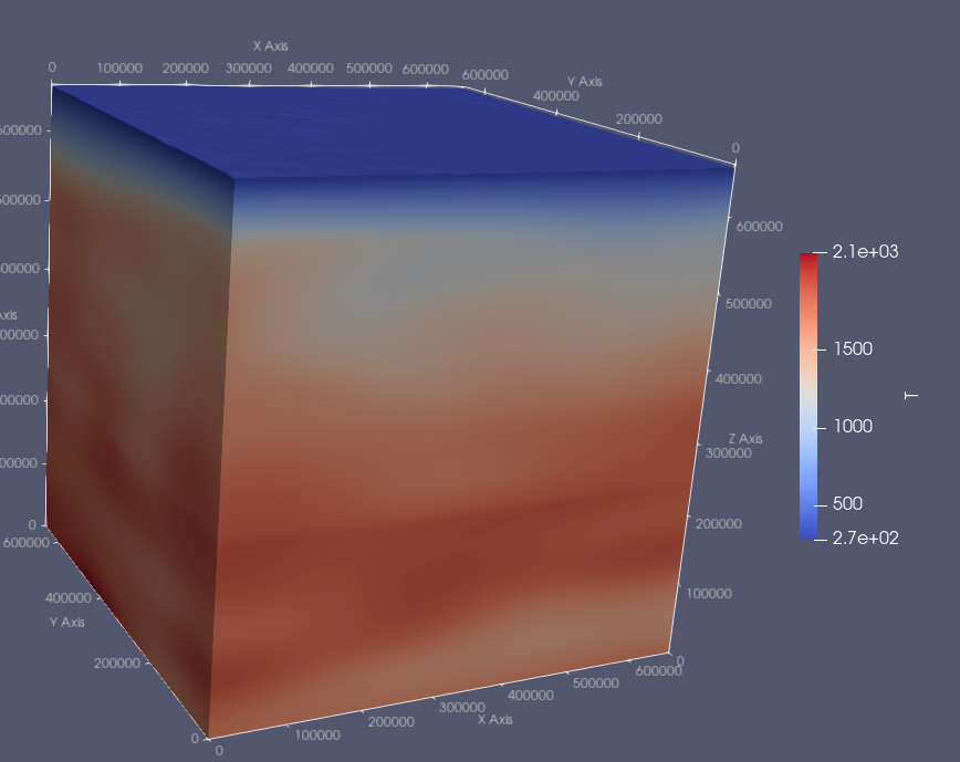
The dynamic topography in my output shows very little spatial variation at each time step..As shown below
I’m not sure whether this is expected behavior or if there’s an issue with my setup.
Additionally, I also tested a diffusion-dislocation material model, and obtained similar results.
The setup is based on the model described in: https://doi.org/10.1093/gji/ggab527
Thanks for your time reading this, and please let me know if there are any other details I can provide!
# x y z dynamic_topography_top
13875 13875 660000 53.54730495
41625 13875 660000 53.09823603
13875 41625 660000 53.47254164
41625 41625 660000 52.96132685
69375 13875 660000 53.11960043
97125 13875 660000 53.13729719
69375 41625 660000 52.96132831
97125 41625 660000 52.96132606
124875 13875 660000 53.14257935
152625 13875 660000 53.12950717
124875 41625 660000 52.9613291
152625 41625 660000 52.96132846
180375 13875 660000 53.09930678
208125 13875 660000 53.05720684
180375 41625 660000 52.96132723
208125 41625 660000 52.953512
13875 69375 660000 53.58243539
41625 69375 660000 52.961326
13875 97125 660000 53.75921824
41625 97125 660000 52.96133022
69375 69375 660000 52.96132632
97125 69375 660000 52.96132639
69375 97125 660000 52.9613321
97125 97125 660000 52.96132905
124875 69375 660000 52.96132873
152625 69375 660000 52.96132728
124875 97125 660000 52.96132917
152625 97125 660000 52.96132764
180375 69375 660000 52.96133
208125 69375 660000 52.95369206
180375 97125 660000 52.96132848
208125 97125 660000 52.96133004
13875 124875 660000 53.98634096
41625 124875 660000 52.96133191
13875 152625 660000 54.19797178
41625 152625 660000 52.9613339
69375 124875 660000 52.96133092
97125 124875 660000 52.96132986
69375 152625 660000 52.96132803
97125 152625 660000 52.96132597
13875 180375 660000 54.30903777
41625 180375 660000 52.96132675
13875 208125 660000 54.29366525
41625 208125 660000 52.96133231
69375 180375 660000 52.96133156
97125 180375 660000 52.96132941
69375 208125 660000 52.96132912
97125 208125 660000 52.96132762
235875 13875 660000 53.02959793
263625 13875 660000 53.00860828
235875 41625 660000 52.95516961
263625 41625 660000 52.95766329
291375 13875 660000 52.99250562

## Initial temperature is from FWEA23 Tomography
set Dimension                              = 3
set CFL number                             = 0.1
set Output directory                     =  nocohension_notopo_novelocity
set Resume computation                     = auto
set Start time                             = 0
set End time                               = 200e3
set Adiabatic surface temperature          = 1600  #K

set Nonlinear solver tolerance                       = 1e-6
set Max nonlinear iterations                         = 500
set Maximum time step                      = 10e3 # Normally set to 20 Kyr
set Surface pressure                       = 0
set Use years in output instead of seconds = true

set Pressure normalization                 = no

set Nonlinear solver scheme                          = single Advection, iterated Newton Stokes
# The `iterated Advection and Stokes' scheme iterates
# this decoupled approach by alternating the solution of the temperature, composition and Stokes systems

#set Maximum first time step                = 10e3
#set Maximum relative increase in time step = 30

# Solver parameters
subsection Solver parameters
  subsection Stokes solver parameters
    set Stokes solver type = block AMG
    set Number of cheap Stokes solver steps = 0
  end
  subsection Newton solver parameters
    set Max Newton line search iterations        = 5
    set Max pre-Newton nonlinear iterations      = 10
    set Maximum linear Stokes solver tolerance   = 1e-2
    set Nonlinear Newton solver switch tolerance = 1e-4
    set SPD safety factor                        = 0.9
    set Stabilization preconditioner             = SPD
    set Stabilization velocity block             = SPD
    set Use Newton failsafe                      = false
    set Use Newton residual scaling method       = false
    set Use Eisenstat Walker method for Picard iterations = true
  end
end


subsection Gravity model
  set Model name = vertical

  subsection Vertical
    set Magnitude = 9.81 # m/s^2
  end
end


subsection Geometry model
  set Model name = box
  subsection Box
    set X extent = 666.e3
    set Y extent = 666.e3
    set Z extent = 660.e3
    set X repetitions = 12
    set Y repetitions = 12
    set Z repetitions = 33
  end
end

subsection Initial temperature model
  set Model name = ascii data
  subsection Ascii data model
    set Data directory       = ./data/
    set Data file name       = temperature.txt #inverted from tomography
  end
end

subsection Boundary temperature model
  set List of model names = initial temperature
  set Fixed temperature boundary indicators   =bottom, top
end


subsection Mesh deformation
  set Mesh deformation boundary indicators = top:free surface

  subsection Free surface
    set Free surface stabilization theta = 0.5
  end
end


subsection Boundary velocity model
   set Tangential velocity boundary indicators =  left, right, front, back, bottom
end

subsection Compositional fields
  set Number of fields = 2
  set Names of fields  = upper_crust, lower_crust
end

# Material model
subsection Material model
  set Model name = visco plastic

  subsection Visco Plastic

    # Reference temperature and viscosity
    set Reference temperature = 273
    set Minimum strain rate = 1.e-19
    set Reference strain rate = 1.e-16

    # Limit the viscosity with minimum and maximum values
    set Minimum viscosity = 1e19
    set Maximum viscosity = 1e24

    set Define thermal conductivities = true
    set Densities = background:3300, upper_crust:2608, lower_crust:2915
    set Heat capacities = background:1250, upper_crust:800, lower_crust:800
    set Thermal conductivities = 3.3, 2.5, 2.5
    set Thermal expansivities = background:3e-5, upper_crust:0.0, lower_crust:0.0

    set Viscosity averaging scheme = harmonic

    set Viscous flow law = composite

    set Grain size = 1e-3
    set Grain size exponents for diffusion creep =        3
    set Prefactors for diffusion creep            = background:2.37e-15, upper_crust:5.00e-51, lower_crust:5.00e-51
    set Activation energies for diffusion creep  =   background:3.75e+05, upper_crust:0.00e+00, lower_crust:0.00e+00
    set Activation volumes for diffusion creep   =   background:1.00e-05, upper_crust:0.00e+00, lower_crust:0.00e+00

    set Prefactors for dislocation creep           =  background:6.52e-16, upper_crust:8.57e-28, lower_crust:7.13e-18
    set Stress exponents for dislocation creep    =  background:3.5, upper_crust:4.0, lower_crust:3.0
    set Activation energies for dislocation creep =  background:5.30e+05, upper_crust:2.23e+05, lower_crust:3.45e+05
    set Activation volumes for dislocation creep  =  background:1.80e-05, upper_crust:0.00e+00, lower_crust:0.00e+00


  #  set Strain weakening mechanism                   = none
  end
end


subsection Initial composition model
  set Model name = ascii data
  subsection Ascii data model
    set Data directory       = ./data/
    set Data file name       = initial_material.txt
  end
end

subsection Boundary composition model
  set List of model names = initial composition
  set Fixed composition boundary indicators = back, front, left, right, top
end


subsection Mesh refinement
  set Initial global refinement          = 0
  set Initial adaptive refinement        = 1
  set Skip solvers on initial refinement       = true
  set Skip setup initial conditions on initial refinement = true
  set Strategy= minimum refinement function
  set Time steps between mesh refinement       = 0
  subsection Minimum refinement function
    set Coordinate system= cartesian
    set Variable names= x, y, z
    set Function constants = CR = 590e3
    set Function expression = if(z>=CR, 1, 0)
  end
end

subsection Checkpointing
  set Steps between checkpoint = 1
end


subsection Postprocess
  set List of postprocessors = visualization, velocity statistics, temperature statistics, topography,basic statistics,dynamic topography
  subsection Visualization
    set List of output variables =stress, strain rate, dynamic topography,maximum horizontal compressive stress,named additional outputs, material properties
    set Time between graphical output = 1e3
    set Interpolate output = true
  end
  subsection Topography
    set Output to file = true
  end
end


subsection Formulation
  set Formulation = Boussinesq approximation
end