Hi everyone, I confused myself when looking into the compressible Stokes system. The momentum conservative equation is given by
\nabla\cdot\left[2\eta\left(\boldsymbol\varepsilon-\frac{1}{3}(\nabla\cdot\boldsymbol u)\boldsymbol 1\right)\right] - \nabla p + \rho\boldsymbol g = \boldsymbol 0,
which is equivalent to
\nabla\cdot\left(\mathbb E : \boldsymbol\varepsilon\right) - \nabla p + \rho\boldsymbol g = \boldsymbol 0.
Here \mathbb E is a fourth-order symmetric tensor. In Voigt notation, \mathbb E can be represented by a 6\times6 matrix:
\mathbb E =
\begin{bmatrix}
\frac{4}{3}\eta & -\frac{2}{3}\eta & -\frac{2}{3}\eta & 0 & 0 & 0 \\
& \frac{4}{3}\eta & -\frac{2}{3}\eta & 0 & 0 & 0 \\
& & \frac{4}{3}\eta & 0 & 0 & 0 \\
& & & 2\eta & 0 & 0 \\
& & & & 2\eta & 0 \\
Sym. & & & & & 2\eta
\end{bmatrix}.
It is easy to see that the sum of the first three rows (or columns) of \mathbb E is 0, which means that \mathbb E is not full-ranked. So why is it possible to invert the top-left block of the Stokes system with CG method?
Another way to see this question is that: for any strain rate with \varepsilon_{xx} = \varepsilon_{yy} = \varepsilon_{zz} \neq 0 and \varepsilon_{xy} = \varepsilon_{xz} = \varepsilon_{yz} = 0, the expression \boldsymbol\varepsilon-\frac{1}{3}(\nabla\cdot\boldsymbol u)\boldsymbol 1 is zero, which means that the kernel space of the top-left block does not only contains 0. Again, it should not be able to be inverted by CG method.
Could anyone help me figure out what goes wrong in my thoughts?
@YiminJin I’ve looked at this for several minutes now already, and I can’t see the fault in your argument. To be specific, the null space of \mathbb E is the Voigt vector (1,1,1,0,0,0), which corresponds to \varepsilon(\mathbf u)=I. This is a purely dilatory strain tensor (corresponding to u=(x,y,z)), and indeed it is not difficult to check that for that, \varepsilon - \frac 13 (\text{trace} \varepsilon) I = 0 in the original (non-Voigt) PDE. Of course, the null space of the operator is bigger than that: It also contains the translations and rotations. It is up to the boundary conditions to pick one element of the null space.
Best
W.
Thank you very much for answering! I did not relate the question to the nullspace corresponding to translation and rotation before, which is eliminated by boundary conditions. It makes a lot of sense.
What I am concerning about is: when the velocity divergence is controlled by some other unknowns, such as in the melt model,
\nabla\cdot\boldsymbol u = -\dfrac{p_c}{\xi},
or in plastic dilation,
\nabla\cdot\boldsymbol u = -\gamma\dfrac{\partial Q}{\partial p},
would it lead to some checkerboard-like patterns like below?
I have observed the checkerboard pattern in plastic dilation problems, but I am not sure whether it is caused by the nullspace. I will check it these days.
Hi @YiminJin ,
There’s a significant chance that I’m talking nonsense in the message below (I play with the plugins, not the solvers), but on the off-chance that it helps…
- Might the mass conservation equation help remove the nullspace of the momentum conservation equation? Density change is directly related to isotropic strain, and density is related to pressure via the equation of state.
- It makes sense to me that the checkerboard patterns that you have observed in the simulations with plastic dilation reflect a nullspace problem. A few of us discussed plastic dilation at the last hackathon, and my understanding was that this dilation could be conceptually viewed as the development of void-space within the model - but that this void space is not treated explicitly in the governing equations. One of the things we discussed was how to prevent runaway dilation, and I wonder whether the dilation and checkerboard patterns might share a common solution.
Best wishes,
Bob
I have no opinion about the models where the divergence of u is determined by some other variable.
But at least for the generic compressible case, as I mentioned above, the null space of \mathbb E is exactly those displacements where \varepsilon(\mathbf u) \propto I. But @bobmyhill is right that the null space of \mathbb E is specifically not in the null space of the second equation of the Stokes equations. In other words, just because there are many velocity fields that satisfy the force balance equation, only one of those also satisfies the divergence equation if you assume that the right hand side of the divergence equation is fixed.
Best
W.
Thank you @bobmyhill and @bangerth ! I agree that the nullspace should be removed by the mass equation if the velocity divergence is constrained by a fixed number, but the problem still exists when the velocity divergence is constrained by a variable. I have been trying to find a solution in the nullspace of
\displaystyle\int_\Omega\left[2\left(\boldsymbol\varepsilon - \frac{1}{3}\nabla\cdot\boldsymbol u\right) - \nabla p\right]{\rm d}\Omega = \boldsymbol 0,
\int_\Omega\left(\nabla\cdot\boldsymbol u + p\right){\rm d}\Omega = 0,
with (\boldsymbol u,p)_{K\in\mathcal T_h}\in Q_2P_{-1}, but I have not found one yet.
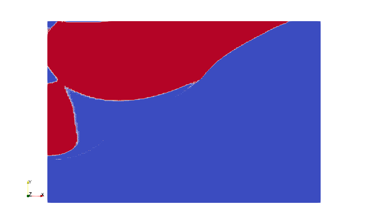
I am also carrying out experiments on the strip-footing model, which I am most familiar with. The good news is that I have found the problem with Picard iteration, and now the Picard method and the Newton method get the same solution:
last year:
now:
I think the PR I submitted last year will be prepared to be merged before or during the Hackathon.
The bad news (not bad for ASPECT) is that the oscillations were not caused by the nullspace. But still, I do not believe this is the best we can get from ASPECT: the shear band is too blurred comparing to other codes.
About the second point raised by @bobmyhill : I do not quite understand the meaning of “runaway dilation”. To me, the checkerboard pattern is something in the plastic_yielding output (look at the edge of the yielding domain):
and I still suspect it has something to do with the nullspace.
Hi @YiminJin,
By “runaway dilation”, I meant the tendency for velocity divergence to continue during prolonged plastic yielding. This is a different problem to the one you are worried about, but I felt that the problems are both related to the decoupling of the density and the velocity divergence.
@YiminJin About the uniqueness: If you have
\nabla \cdot u = \alpha p
(note the different sign compared to your equation), you have a problem for which you can prove uniqueness of velocity and pressure with the same techniques as for the Stokes equations. Perhaps easier is the following approach: For \alpha>0, algebraically, the equations above lead to a matrix of the kind
\begin{pmatrix} A & B^T \\ B & -\alpha M \end{pmatrix}
for which the Schur complement is S = B^T (\alpha M)^{-1} + A, which is a positive definite and symmetric matrix because M is symmetric and positive definite, and A is symmetric and positive semidefinite. This guarantees unique solvability for the velocity. Once you have the velocity, you then use the second equation to solve for p, which is again a unique solution because M is positive definite.
Best
W.
Hi @bobmyhill ,
I have not met the situation you described. From my understanding, plastic dilation is a response to the pressure increase when the dilation angle is greater than 0. It can be explained by a sketch:
In the figure above, \phi and \psi are the friction angle and the dilation angle, respectively. When \psi=0, the trial stress \boldsymbol\sigma^{\rm tr} is mapped onto the yield surface with no change in pressure; when \psi>0 (in this specific case, \psi=\phi), the return-mapping is accompanied with a pressure increase. The dilation is induced by the extra pressure.
However, this is only a conceptual description in the principal stress space. We can also assume that the extra pressure is induced by the void-space created by plastic yielding, as you mentioned. It is like a chicken-or-egg problem. Honestly, I do not fully understand the physics of plastic yielding, and why the non-associated flow rule breaks the ellipticity of the problem. Please let me know if I make mistakes in my statements.
Best,
Yimin
Hi @bangerth ,
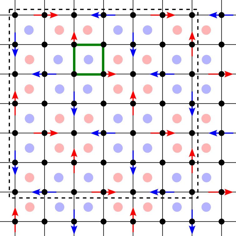
Thank you for providing help in proving the uniqueness of the solution! I did not find mistakes in your proof. However, I confuse myself again because I think I have found a non-trivial solution in the nullspace of the compressible Stokes equation:
The solution is in Q_1P_0 space (and also in Q_2P_{-1} space). The arrows denote the velocity at each node, and the circles denote the pressure in each cell. If there is no arrow/circle, then the velocity/pressure on that node/cell is zero. It is easy to see that the solution is consistent with free-slip boundary condition (for example, if the model only contains the cells within the dashed lines).
Since the velocity state in each cell is similar, we only need to analyze one of them. Take the one in green box for example. Its velocity field is:
\boldsymbol u =
\begin{bmatrix}
x(1-y) \\ (1-x)y
\end{bmatrix}.
Its strain rate is:
\boldsymbol\varepsilon =
\begin{bmatrix}
1-y & -\frac{1}{2}(x+y) \\ -\frac{1}{2}(x+y) & 1-x
\end{bmatrix}.
The deviatoric strain rate is (here we use 1/2 instead of 1/3 to mimic the situation in 3D):
\boldsymbol\varepsilon - \dfrac{1}{2}(\nabla\cdot\boldsymbol u)\mathbf 1 =
\begin{bmatrix}
\frac{1}{2}(x-y) & -\frac{1}{2}(x+y) \\ -\frac{1}{2}(x+y) & \frac{1}{2}(y-x)
\end{bmatrix}.
Then it is easy to verify that
\nabla\cdot\left[\boldsymbol\varepsilon - \dfrac{1}{2}(\nabla\cdot\boldsymbol u)\mathbf 1\right] =
\boldsymbol 0 = \nabla p.
Note that the expression above is not zero if the volumetric part is not subtracted.
For the mass equation, there is always a p satisfying
\displaystyle\int_K(\nabla\cdot\boldsymbol u - \alpha p){\rm d}\boldsymbol x = 0
in Q_1P_0 space, no matter if \alpha is positive or negative.
Is there something wrong in my derivation?
Best,
Yimin
@YiminJin I did not check the details, but I want to note that the choice of the factor 1/2 to denote a 2d situation is difficult. We typically think of 2d situations as one where there is a third z dimension but things are constant in z direction. In that case, you need to continue to use 1/3 in the equations, even though you’re doing a 2d simulation. Using 1/2 implies that you are modeling a specific situation that is different from a 2d cross section of an infinite 3d domain. I believe that there is a substantial section on this issue in the part of the ASPECT manual that describes the equations being solved.
Best
W.
Hi @YiminJin ,
My message below is from a physical perspective rather than a purely mathematical one, but perhaps it’s still useful.
The pattern you’ve drawn looks like a superposition of two orthogonal standing waves (e.g. https://physics.stackexchange.com/questions/69587/how-to-add-two-plane-waves-if-they-are-propagating-in-different-direction). The main difference between a standing wave and your sketch is that the velocities in your sketch are in-plane, not out-of-plane.
I think it’s helpful to ask what conditions are required for such a pattern to physically exist. Standing waves in elastic media require (a) sufficient energy in the system, (b) a material capable of storing and transferring energy between elastic potential and kinetic energy, and (c) initial conditions or perturbations tuned to the resonant modes of the system. Elastic energy is quadratic in strain, so small waves can appear in an initially static but noisy domain, but they cannot grow without at least a source of energy.
A plastic system should be constrained in analogous ways. An emergent pattern of alternating compression and dilation like the one you have drawn is possible only if no energy is required to drive the deformation. But plastic deformation requires the presence of finite deviatoric stresses and is inherently dissipative. For this reason, I do not think that a realistic implementation of plastic deformation should produce deformation like that which you have shown.
Best wishes,
Bob
Hi @bangerth and @bobmyhill ,
Thank you for looking into my question and pointing out my mistake. I have tried to extend the pattern to 3D case but it no longer satisfies the equation. Furthermore, I tried to replace the term -\frac{1}{3}(\nabla\cdot\boldsymbol u)\boldsymbol 1 by \frac{1}{3}\gamma\frac{\partial Q}{\partial p}\boldsymbol 1 in plastic dilation problem, and the solution is even worse than the original form (there is no oscillation, but the strain concentration is so weak that there is no shear band formed).
I think I need to do some literature research about this problem. I started focusing on this problem because I have found strange oscillations in strain rate field and a severe drop in convergence rate when solving the compressible Stokes system, but the problem may not relate to the nullspace. I hope to see if there are other people encountered with the same problem in the past.
Thank you again for spending time on this!
Best wishes,
Yimin