Issues with ASPECT model for subduction initiation

[Ozias]

Hello every one,

I hope this message finds you well.

My name is Vladmir, and I am currently working on a project using ASPECT to model subduction initiation triggered by the collision of two continents. I have been reviewing the ASPECT cookbooks and benchmarks for guidance on building my input file, but I’ve encountered a few challenges along the way and would appreciate any insights you might have.

My model includes 8 compositional fields, and the oceanic lithospheric mantle’s temperature is governed by half-space cooling. The viscosity range I’m working with spans from 1e20 to 5e23 . I’m using a viscoplastic rheology combined with a composite viscous flow law. However, the model solving fails after the first time step when the composite law is used.

When I attempt to run the model with only dislocation or diffusion creep, it begins to run, but I encounter an error later in the simulation indicating that the iterative solver is not converging.

Additionally, I’ve noticed that the initial time step starts high but drops significantly after a short time, eventually reaching values close to one year. This presents a problem given that the end time for my simulation is set to 22 million years.

I would greatly appreciate it if someone could assist me in handling these issues. Any help or suggestions would be invaluable.

Thank you for your time and assistance.

Best regards,
Vladmir

[bangerth]

@Ozias
Would you mind showing us the error message you get? Being specific is always useful, rather than just saying “I get an error” because we cannot guess what that error is.

I would not be surprised if the two issues you mention are related. If your model ends up with regions where the viscosity becomes small, then the velocities will be large, and that will trigger a small time step. Generally, linear solvers will often fail if you have too large a range for the viscosities. So I would output the viscosities into the visualization files, and take a look at that during the last time step in which the solver succeeds. You can also output the maximal velocity (as part of the “velocity statistics” postprocessor) to see whether my hunch above is correct.

Best
W.

[Ozias]

Hi @bangerth,
Thank you for your quick response. it’s really appreciated.
I’ve taken note of your feedback.
Attached are the screenshots of the last time step and the error, as well as the prm file.

initiation.prm (8.4 KB)

[bangerth]

Oh, I see, it’s one of the advection variables for which the solver fails. That’s interesting. I’m not sure I’ve seen that. Can you show how the clc variable (the one for which the solver fails) looks like in the previous time step?
Best
W.

[Ozias]

Dear @Bangerth,

I hope this message finds you well.

I have attached a snapshot that highlights the appearance of the continental lower crust (clc) variable in the two previous time steps. Additionally, I’ve included the PRM file with comments. My apologies for not including the comments in the initial file I sent.

I truly appreciate your willingness to take a look at this. Thank you for your continued support

subduction_initiation.prm (9.9 KB)
.

Best regards,
Ozias

[bangerth]

@Ozias What I meant is can you show us a visualization of the variable at the previous time step?
Best
W.

[Ozias]

Sure @bangerth.
Here is how it looks like.

Some of the compositional fields, such as cuc and ouc, are not being solved, as seen in the previous snapshots I shared. However, I believe this can be addressed by refining the mesh.

I’ve also tried adjusting various parameters in the material model, solver, and global settings throughout the day, but I always run into convergence issues.

Best,
Ozias

[jbnaliboff]

Hi @Ozias,

I’m jumping into this discussion late, but wanted to add on to a few of the comments and suggestions from @bangerth.

I agree with Wolfgang’s assessment that the issue is related to the time steps being too large (there are likely a number of related issues as well). The very small time steps you are seeing prior to the model crashing is not surprising, given that you have a free a surface and the model is likely undergoing some degree of isostatic adjustment initially (other factors can lead to low velocities as well).

This is a common feature of models with subduction initiation in combination with a free surface and laterally varying lithospheric properties.

Here are some suggestions to start:

1. Systematically start decrease the CFL value (currently set to 1) to see if this resolves the issue. My guess is a value on the order of 0.1 or 0.2 is needed for this type of problem. An even lower value might be needed to
2. Use a stricter linear solver tolerance (1e-7 or 1e-8) for the Stokes system, to ensure there are no unphysical velocity anomalies producing advection solver errors.
3. Use a nonlinear solver scheme (iterated Advection and Stokes) and stricter nonlinear solver tolerance (1e-4 to start), which may help stabilize the system.
4. If you have not already done so, try running the models with a free-slip top boundary and then once move onto models with a free surface once you are satisfied with the results.

If you have not already seen it, the following paper looking at subduction dynamics using ASPECT might be a good reference for model design or re-building the models from scratch (if needed) - Behr et al. (2022). This is at least where a student and I started from recently when building 2D subduction simulations.

Cheers,
John

[Ozias]

Dear @jbnaliboff,

It’s a pleasure to have you in this discussion, and I sincerely appreciate your valuable suggestions. I will implement them and explore the outcomes.

The paper you shared is truly fascinating; it’s one of the first I’ve come across that provides this kind of detailed breakdown of how the .prm file was constructed. Most papers I’ve encountered typically briefly focus on governing equations, numerical model, and material rheology without delving into these practical aspects. If you have any other recommendations for similar papers, I would greatly appreciate them.

Thank you again for your insightful guidance, and I’m also grateful to @bangerth for the support. I’ll get back to you as soon as I have updates.

Best regards,
Ozias

[Ozias]

Hi @jbnaliboff,

I hope you’re doing well!

I’ve been implementing your recommendations and have made some
interesting progress. I also defined the parameters for plasticity,
which has contributed to better results. However, I’m still working on
properly defining the initial temperature model.

The initial composition model consists of:
A continental plate, a micro-continent, and two oceanic plates. One
is already subducting beneath the continental plate., and the other is
located to the left of the micro-continent, with a weak zone in the
middle for subduction initiation.

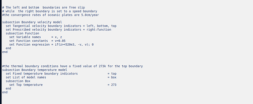
Initial temperature model:
- In continental regions, temperature increases from 273K to
1573K in thermal equilibrium.
- In the oceanic mantle lithosphere, temperature is controlled
by half-space cooling.
- In the asthenosphere, I initially set a temperature gradient
of 273.5K, but defining a proper temperature distribution is
challenging due to the irregular lithosphere-asthenosphere boundary
(LAB) and varying temperatures at the base of each lithosphere.
For now, I’ve set a uniform 1375K temperature in the asthenosphere as
a temporary solution.

I reviewed the paper you previously shared and noticed they used
additional Python plugins for temperature initialization. However, I’m
not familiar with implementing Python plugins in ASPECT yet. If anyone
has insights on defining the temperature field directly within ASPECT,
I would really appreciate any guidance!.

Issues I’m Facing when i get some outputs with the initial
temperature i assumed:
I. Low Resolution in Output Visualizations
1. The viscosity variable does not display anything useful
when visualized.
2. Some compositional fields do not appear in the output
(even when RHS = 0).

 II. Mesh Refinement & Solving Time Issues
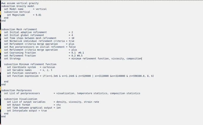
        When I adjust mesh refinement settings, the solver

struggles with performance. And the minimum refinement is not helping
in my case at all.
Even with adaptive refinement = 2 and global refinement =
4, the solving time is extremely slow (taking at least 10 minutes per
time step).

  III. Model Dynamics Issue
     When I try to run the model, nothing moves, only the

resolution deteriorates over time. I’m running the .prm file with 4
processors.
I’ve attached below some snapshots of the input file and how the
initial temperature model and the viscosity variable look like in the
first output I got.

I’d appreciate any suggestions on improving the initial temperature
model and mesh refinement settings to make the solver run more
efficiently.
Thanks in advance for your help!

Best,
Ozias

(attachments)

[jbnaliboff]

Hi @Ozias,

My guess is that the Behr et al. paper used python scripts to create initial temperature distributions that were written to an ascii file, which were then read by ASPECT to define the initial temperature (this is currently an option).

I think the easiest approach would be to use the geodynamic world builder to define the initial conditions (temperature and composition).

This open pull request illustrates the approach, and I believe that this will get updated soon based on recent improvements from @daniel.douglas.

My recommendation is to start from these files (but remove the reactive fluid flow components) and test different initial setups with the GWB until the pull request is updated.

Cheers,
John

[Ozias]

Dear @jbnaliboff,

Thank you for your prompt response. It’s reassuring to see how much all of you care about ASPECT users, which is truly encouraging.

I will implement the new recommendations you provided and look forward to seeing the results.

Regarding mesh refinement, do you have any suggestions ?

Thanks again for your assistance.

Best regards,
Ozias

[jbnaliboff]

@Ozias,

Regarding mesh refinement, do you have any suggestions ?

For this class of problems the maximum resolution should be at least 4-5 km resolution, but it is of course highly case dependent. In the end, some of these decisions will be governed by what resources you have access to. I would start with the settings in the pull request above, and then decrease the resolution if it is too computationally intensive.

Cheers,
John

[Ozias]

Hi everyone!

I hope you’re all doing well. I just wanted to provide an update on my model and ask for some help. Right now, the main issue is with visualizing the viscosity variable. When I first get the output, the compositional fields are very skewed. When I switch to a log scale for visualization, I see that the viscosity is unusually high in the asthenosphere.

I’ve gone through some of the previous discussions in the community and tried to implement the suggested solutions, but unfortunately, the issue persists. The solutions I tried were related to material averaging, viscosity averaging schemes, nonlinear solver schemes, and solver parameters, but none of them seem to work.

Initially, as I mentioned, the output isn’t visualized well, but as I run the model, it starts to improve. So, I thought I’d keep it running in hopes that, over time, the viscosity variable would eventually show up as expected. Unfortunately, I ran into convergence issues. To fix this, I’ve adjusted the CFL number (tried values like 0.05, 0.1, 0.2, 0.3, 0.5), the nonlinear solver iterations (1e-2, 1e-3, 1e-4, 1e-5), the linear solver tolerance (1e-5, 1e-6, 1e-7), and the maximum linear Stokes solver tolerance (values like not defined, 1e-1, 1e-2, 1e-3). I also fine-tuned the mesh refinement parameters, but nothing seems to allow the model to run as expected.

I’ve attached some screenshots to provide more context.
Looking forward to any suggestions or help you might have!

Best,
Ozias

1. Density variable to show how the model should look like
   

   

2. Initial visualization (both ordinary and log scale)
   

   
   
   
   

3. Output after 27,000 years (ordinary and log scale)
   

   
   
   
   

4. PRM file
   

   
   
   
   
   
   
   
   
   
   
   
   
   
   
   
   

5. Last time step
   

   

[Ozias]

Dear @all,

I hope this email finds you well. I would like to follow up on the issue I previously encountered with my model.

Currently, I have managed to run the model for a time of 7e6 years. However, I am still facing a convergence problem. The viscosity issue remains unresolved, and the model stays stationary throughout the entire runtime.

I also attempted to run the model in debug mode, but I encountered a floating-point error. I have attached the relevant snapshots of the .prm file, as well as the error obtained during the debug run.

I would appreciate any insights or suggestions you may have regarding this issue.

@jbnaliboff, @wolfgang Bangerth

Thank you for your time!

Best regards,
Ozias

[jbnaliboff]

Hi @Ozias,

Sorry for the delay in responding to last series of questions.

To summarize, there a number of issues:

1. Unexpected viscosity values in the asthenosphere
2. Convergence issues for the advection solvers.
3. Floating point errors when running in debug mode

Some or all of these issues are likely related.

The model results you posted above have fairly complex initial conditions, and it will be quite hard to diagnose all of the potential issues.

It may seem like a step backwards, but I think the best approach is to start with a much simpler model (i.e., similar to the Behr et al. paper mentioned above or Grima and Becker, 2024) and systematically build up complexity.

Cheers,
John

[bangerth]

I second @jbnaliboff 's suggestion. In general, if you get an error in debug mode, it is not useful to believe that you get anything useful in release mode. Just because the code makes it past the error in release mode does not mean that the error was meaningless and can be ignored. The right approach is to find out why you get the error, and then fix that.
Best
W.

[Ozias]

Hi @jbnaliboff & @bangerth,

I really appreciate your quick and helpful responses! I’ll try out your suggestions and let you know how it goes.

Best,
Ozias