Hi,
The output of the Pylith example is almost displacement. I would like to build a 3D fault model to simulate the rate of interseismic deformation at the surface. I have tried several times without success. Can you please help me if you know how to do it?
To compute the rate of interseismic deformation, you need to create a model that has variation in deformation over time. For example, you could impose velocity boundary conditions with a linear elastic rheology. You can compute an average rate by dividing the displacement by time. If you include viscoelastic rheologies, then you may need to run your model for many time steps to find the steady state solution. We might be able to provide more help if you provide a diagram of the boundary value problem you are trying to solve.
It’s unclear exactly what you want. If you want the velocity field at the surface you would need to do a little post processing. PyLith outputs the total displacement field, so to get velocities you would need to compute the displacement differences between one time step and the next, and then divide this by the time step size. This is easy to do with a simple Python script (using h5py and numpy). If you want the strain rate field you would need to do something similar with the total strain output from PyLith.
Here are all the files for my simulation using Pylith, including the finite element model, Pylith control scripts, rheological parameter settings, output files, etc. We want to output the surface deformation rate, and after trying for some time we still can’t succeed.
I think your may be having trouble because you include the velocity field in the solution. The quasistatic formulation does not use the velocity field in the solution; it is used in the dynamic (include inertia). See equation 114 at Quasistatic — PyLith 4.0.0 documentation. As Charles and I have suggested, you should use the displacement field and you can divide by time to get a velocity or rate of deformation.
I am interested in calculating the rate of interseismic deformation. I applied elastic rheology on top of viscoelastic rheology with a vertical fault embedded in the elastic rheology. I applied a velocity boundary condition on the model block sides. However, I am a bit confused about how to achieve the steady-state solution. Is the steady state solution archived when the fault fails (If I use friction on the fault)?
A steady state is reached when the deformation as a function of time approaches a velocity field that remains relatively constant over time. In most cases for a boundary value problem with fault friction, it means either there is steady sliding or cyclic fault slip.
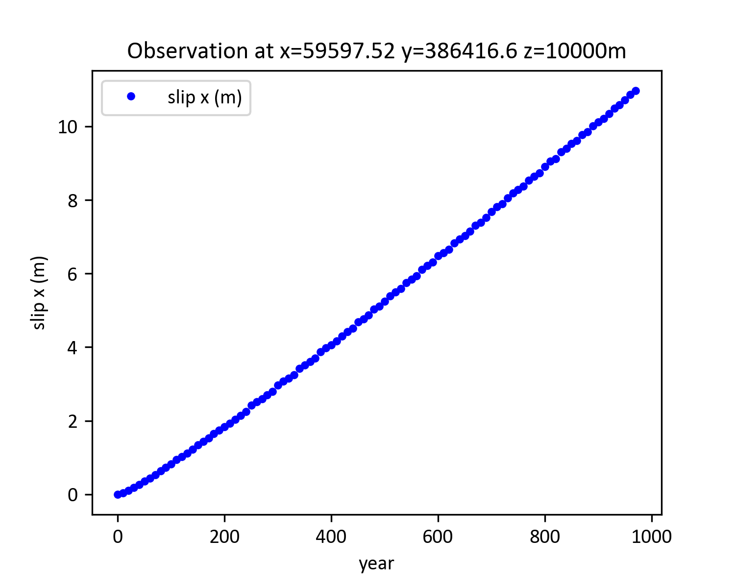
I tried to estimate the fault slip rate, by running the aforementioned model for 1000 years (timestep 10). The model is a vertical fault (0-30km) embedded in elastic layer (0-30km), underlaid by viscoelastic material (30-80km). The fault has friction 0.1, cohesion 2 MPa, and Static Friction were used. The model successfully ran for 1000 years.
I attempted to estimate the fault slip rate by calculated the delta of slip at consecutive timestep (e.g. [slip x at time step 20 - slip x at time step 10] / 10 years). But when I plotted it on a graph, the slip rate does not show smooth trend, but shows fluctuated trend (as shown after year 100, in left figure below).
Is it ok to have the trend like this? Does the line after year 100, considered as the steady state phase?
Kindly advise.
Below is the figure showing fault slip x, at observation point (x=59597.52, y=386416.6) on the fault, and estimated slip rate. Thank you.
The slip rate can vary in time for a variety of reasons. There may be complex spatial variations due to interactions across the fault, especially if the fault is non-planar, which results in spatial variations in the fault-normal tractions. I would test whether these features are sensitive to the discretization size along the fault. That is, if you run simulations with finer and coarser resolutions along the fault, do you obtain similar results? Obviously, this type of model is a simplification of the physics, so the results should be analyzed and placed in the proper context with respect to observations and inference of behavior.